SVGF (Spatiotemporal Variance Guided Filtering)
This is a simple implementation of Spatiotemporal Variance-Guided Filtering.
I extended a cuda path tracer that I wrote to build it.
It denoises 1 sample per pixel path tracing outputs in real time (~6ms)
It’s using openGL for rasterizing the scene and cuda for ray tracing. The raytracing backend can either use a custom BVH implementation, or NVidia optiX.
It’s not a complete implementation, for example it’s not doing albedo demodulation as described in the paper, so it doesn’t really work with textured meshes.
It’s also not really optimized, although the filtering part is quite fast, the path tracing part could be faster, but my focus was more on implementing the filter rather than speeding up the path tracer.
SVGF
There are 5 main steps in the algorithm that I will detail here :
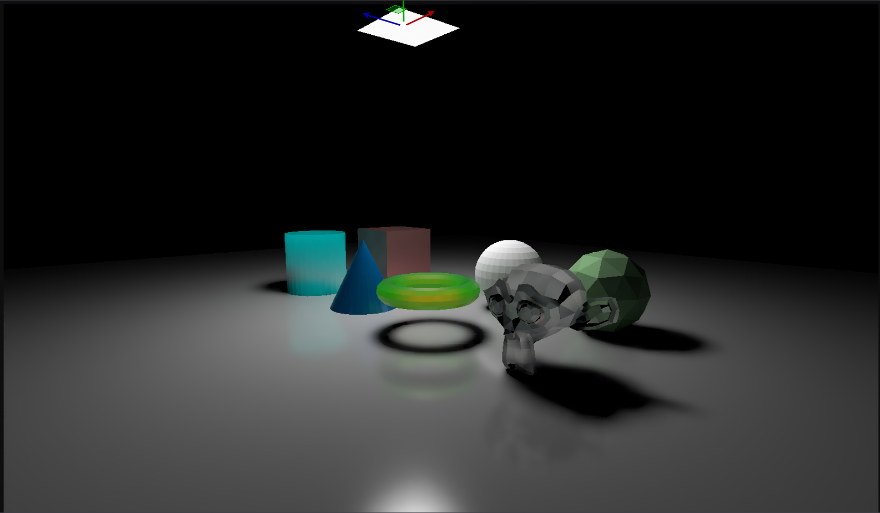
1. Rasterization
In this part, we simply rasterize the scene in a framebuffer that contains multiple render targets :
-
Render Target #1 : This contains the 3d position of the fragment, and the triangle index in the alpha channel
-
Render Target #2 : This contains the world normal of the fragment, and the material index in the alpha channel
-
Render Target #3 : This contains the triangle barycentric coordinate of the fragment, and the instance index in the alpha channel
-
Render Target #4 : This contains the 2d motion vector of the fragment in the rg channels, and the linear depth and depth derivative in the ba channels.
Motion vectors are calculated by taking the previous camera view matrix, calculating where this fragment was in the previous frame, and taking the difference between the current and previous pixel positions.
The depth is simply the distance between the camera and the fragment world position, and the depth derivative is calculated using dFdX/Y functions in glsl.
Note that we’re using a double framebuffer approach here, like in most of the subsequent steps too.
This means that we actually have 2 openGL framebuffers, and every frame we swap the framebuffer to which we render. This allows to keep track of the previous frame output at all times, which will be handy for the calculations that we need to do later on.
Here’s how we create those framebuffers :
    std::vector<framebufferDescriptor> Desc =
    {
        {GL_RGBA32F, GL_RGBA, GL_FLOAT, sizeof(glm::vec4)}, //Position
        {GL_RGBA16UI, GL_RGBA_INTEGER, GL_UNSIGNED_SHORT, 4 * sizeof(uint16_t)}, //Normal
        {GL_RGBA16UI, GL_RGBA_INTEGER, GL_UNSIGNED_SHORT, 4 * sizeof(uint16_t)}, //Barycentric coordinates
        {GL_RGBA32F, GL_RGBA, GL_FLOAT, sizeof(glm::vec4)}, //Motion Vectors and depth
    };
    Framebuffer[0] = std::make_shared<framebuffer>(RenderWidth, RenderHeight, Desc);
    Framebuffer[1] = std::make_shared<framebuffer>(RenderWidth, RenderHeight, Desc);
and how we bind them :
Framebuffer[PingPongInx]->Bind();
...
PingPongInx = 1 - PingPongInx;
Here, PingPongInx always contains the index of the current frame framebuffer, and 1 - PingPongInx contains the previous frame’s framebuffer. At the end of the current frame, we do PingPongInx = 1 - PingPongInx to swap.
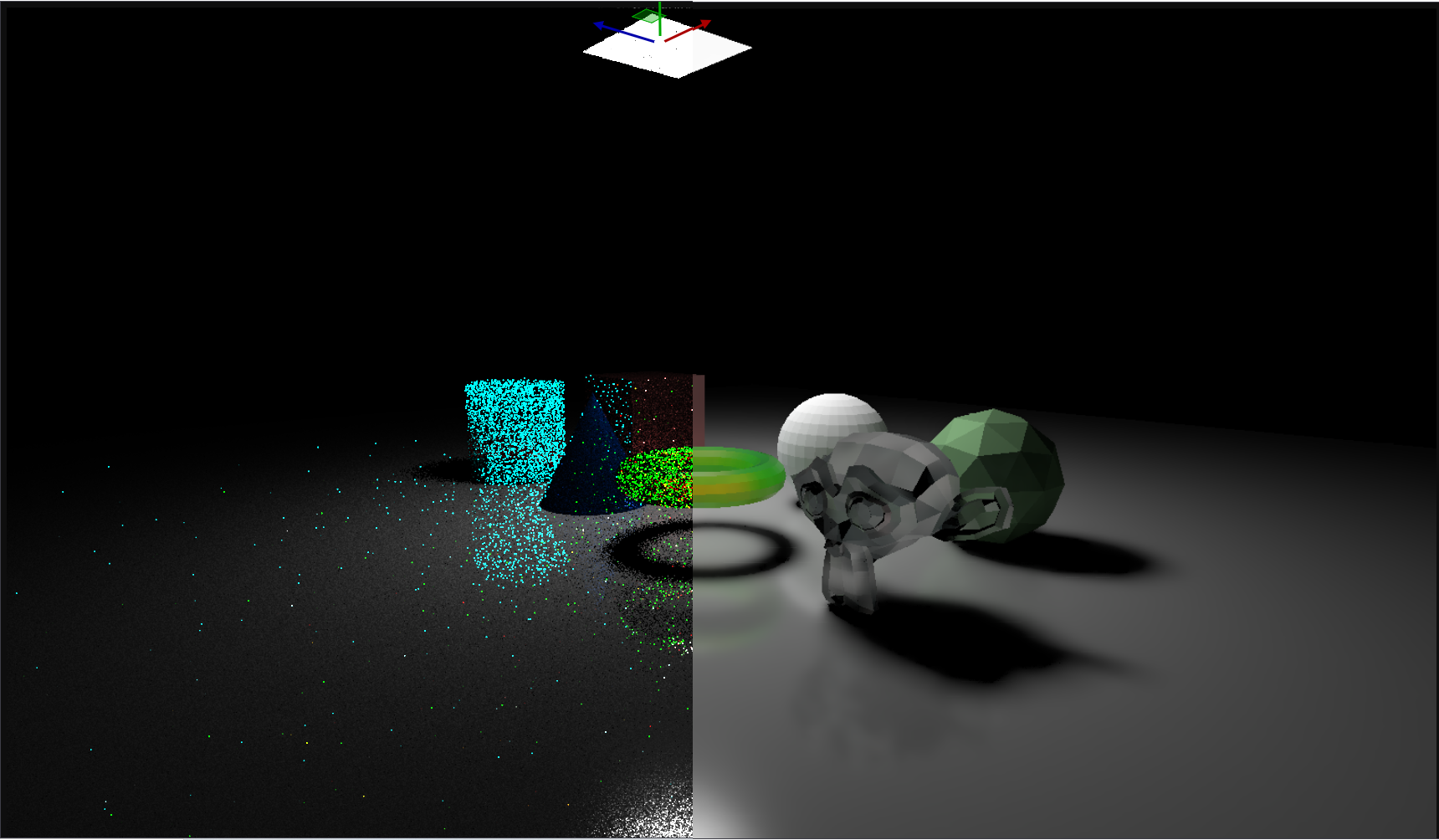
2. Path Tracing
In this step, we use the geometry buffer that’s output by the rasterization step as a baseline for operating a 1 sample per pixel path tracing.
Note that using the geometry buffer is not necessary, and SVGF can also work with fully path traced pipelines, but I wanted to test this “hybrid” approach and see how it performs.
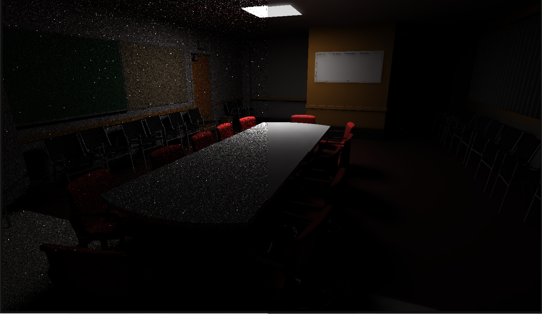
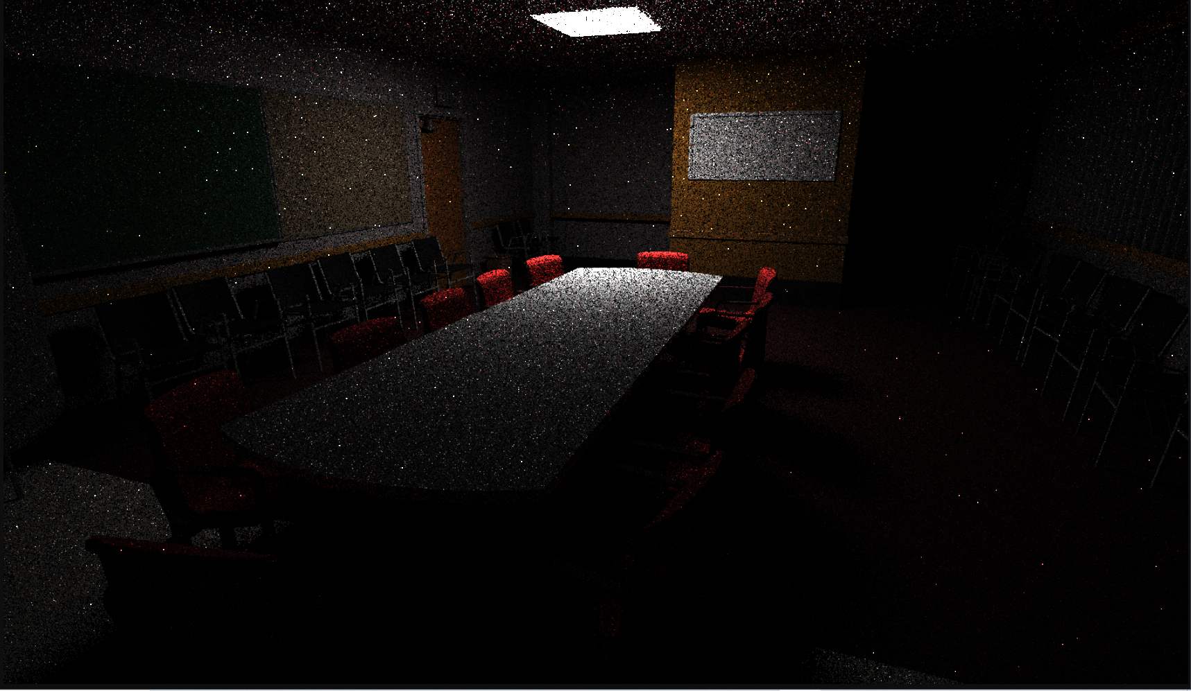
The output of this step is a noisy image like that :
Here again, we use double buffers, meaning we can keep track of the previous frame output.
3. Temporal filtering
In this step, we will be accumulating the results from previous frames using an Exponential moving average, which will already remove some noise
To do that, for each pixel in the rendered image, we check if we can retrieve it in the previous frame. If the camera hasn’t moved, it’s easy, that pixel will be at the same position.
If the camera has moved, we need to use the motion vectors to retrieve it in the previous frame, and we need to check that the value that we read from the previous frame is correct.
Indeed, if the pixel was disoccluded, we won’t find its previous value in the previous frame.
the exponential moving average is implemented using a “History Buffer”, which for each pixel stores how many frames are accumulated for that specific pixel.
Here’s how it works :
    bool CouldLoad = LoadPreviousData();
    if(CouldLoad)
    {
        HistoryLength = min(HistoryBaseLength, HistoryLength + 1 );
        Alpha = 1.0 / HistoryLength;
    }
    else
    {
        Alpha = 1;
        HistoryLength=1;
    }
    vec3 NewCol = mix(PrevCol, CurrentColour, Alpha);
For each pixel, we try and load its previous data. If we can load, then we increment the history length, and set the interpolation factor to be the inverse of that.
If we can’t load, then alpha is naturally 1 as we don’t want to interpolate with the previous frame, and we reset the history length to 1.
That’s all for colour temporal accumulation.
But in this step, we can also compute some values that will be needed for later steps, namely the “variance” and the “moments”
The “First Moment” represents the average brightness of the pixel, so it’s like an average of the luminance of that pixel.
The luminance can be calculated as follows :
float CalculateLuminance(vec3 Colour)
{
    return 0.2126f * Colour.r + 0.7152f * Colour.g + 0.0722f * Colour.b;
}
The “Second Moment” involves squaring the luminance values before averaging them. It captures more information about the distribution, particularly how spread out the values are.
Here’s how we calculate the 2 moments :
Moments.x = CalculateLuminance(CurrentColour);
Moments.y = Moments.r * Moments.r;
Moments = mix(PreviousMoments, Moments, Alpha);
Finally, the variance is calculated by substracting the square of the first moment to the second moment :
float Variance = max(0.f, Moments.g - Moments.r * Moments.r);
Here, a high variance will indicate that there’s some noise on that pixel, which will be handy when filtering the noisy output (Hence the “Variance Guided” part in the title)
In the paper, they also demodulate the albedo from the image, so that the later steps only work on white surfaces. This is because if there are textured surfaces, we don’t want the filter to blur those colours.
I haven’t done that but it shouldn’t be too difficult to add.
4. A-Trous Filter
In this step, we’ll be filtering the noisy output using an “A-trous wavelet filter”.
This filter is ran multiple iterations, each time with an increasing radius or “step size” (1, 2, 4, 8, 16…) :
    int PingPong=0;
    for(int i=0; i<SpatialFilterSteps; i++)
    {
        filter::half4 *Input = (filter::half4 *)FilterBuffer[PingPong]->Data;
        filter::half4 *Output = (filter::half4 *)FilterBuffer[1 - PingPong]->Data;

        int StepSize = 1 << i;

        filter::FilterKernel<<<gridSize, blockSize>>>(Input, Framebuffer[PingPongInx]->CudaMappings[(int)rasterizeOutputs::Motion]->TexObj, Framebuffer[PingPongInx]->CudaMappings[(int)rasterizeOutputs::Normal]->TexObj,
            (uint8_t*)HistoryLengthBuffer->Data, Output, (filter::half4*) RenderBuffer[PingPongInx]->Data, RenderWidth, RenderHeight, StepSize, PhiColour, PhiNormal, i);

        PingPong = 1 - PingPong;
    }
This is the most complicated part of SVGF, but I’ll still try to explain what happens.
For each pixel, we will iterate through its neighbouring pixels, like we would do for blurring an image for example.
we will take a 5x5 neighbourhood around the pixel, but remember the step size increases ! For the first iteration, the step size is 1, so we really do take the 5x5 neighbourhood :
x x x x x
x x x x x
x x o x x
x x x x x
x x x x x
Here, “o” is the current pixel, and “x” are all the samples that we’re checking in the surroundings of o. “_” are other pixels that we’re not checking.
But for the second iteration, where stepSize is 2, we go further in the neighbourhood :
x _ x _ x _ x _ x
x _ x _ _ _ x _ x
x _ x _ x _ x _ x
x _ x _ _ _ x _ x
x _ x _ o _ x _ x
x _ x _ _ _ x _ x
x _ x _ x _ x _ x
x _ x _ _ _ x _ x
x _ x _ x _ x _ x
Here’s the code that does that :
   for (int yy = -2; yy <= 2; yy++)
    {
        for (int xx = -2; xx <= 2; xx++)
        {
            vec2 CurrentCoord = FragCoord + ivec2(xx, yy) * Step;
            ...
        }
    }
Great, so what do we do with those neighbouring pixel values now ?
well, we use them to apply a “cross bilateral filter”, and to do that, we will use an “edge stopping function”.
Here I’ll briefly explain what a bilateral filter is and how it works.
Bilateral filters are used in image processing to smooth images while preserving edges, meaning we can remove noise in rather “flat” areas and keep the sharp edges intact.
To do that, we loop through all the neighbouring pixels, and take into account both the distance of the neighbourg pixel to the central one, and the change in intensity between the two.
This means that pixels closer to the central pixel will usually have a higher weight, and pixels with similar intensities to the central pixel will also have a higher weight.
We therefore have to calculate a “spatial” and an “intensity” weight that we then multiply together to get the weight of a neighbour pixel.
For each neighbour, we calculate the weight of that neigbour, and multiply it with its pixel value. We accumulate that over all the neighbourhood, and finally we divide by the sum of all the weights to normalize the value.
the term “cross” bilateral filters means that we use another image to drive the weights of the filtered image. In this case, we use the variance image and the geometry buffers to do so.
Now that we reviewed what a bilateral filter is, we will explain how the SVGF specific filter will work, and how we calculate the weights.
The filter is described in equation (1) of the paper, and here’s a pseudo code implementation of that equation :
SumColour
for each pixel q around pixel p  :
    kernelWeight = kernelWeights[q] //Those are [3/8, 1/4, 1/16]
    edgeStoppingWeight = CalculateEdgeStoppingWeight() //This is the complicated function !
    pixelWeight = kernelWeight * edgeStoppingWeight

    SumColour += pixelWeight * Colour[q]
    SumWeight += pixelWeight

FilterOutput = SumColour / SumWeight
So now, what does this CalculateEdgeStoppingWeight() function looks like ?
Well, it uses geometrical (world normals and depth) and luminance information to calculate a weight.
That weight is defined as a product of 3 weights : Depth, Normal and luminance.
- Normal : This is described in equation (4) of the paper, and here’s the code :
const float weightNormal = pow(max(dot(normalCenter, normalP), 0), phiNormal);
- Depth : This is described in equation (3) of the paper, and here’s the code :
float Numerator = abs((zCenter.x - zPixel.x)); float Denominator = max(abs(zCenter.y), 1e-8f) * Step; //Here, sigma_z is 1, and step represends (p-q) : the distance between the 2 pixels. float weightZ = exp(-(Numerator / Denominator)); - Illumination : This is described in equation (5) in the paper, and here’s the code :
float Denominator = SigmaLuminance * sqrt(max(0, 1e-10 + Variance)); //Here, this is the prefiltered variance
float weightLillum = abs(luminanceIllumCenter - luminanceIllumP) / Denominator;
Note that for the illumination and depth weights, we didn’t put them in the exp(-) as described in the equations.
Instead, we do that all in one go when computing the final weight, as an optimization :
const float weightIllum = exp(0.0 - max(weightLillum, 0.0) - max(weightZ, 0.0)) * weightNormal;
This will result in a weight that will preserve the edges in the output images, and blur otherwise, which is exactly what we want.
Note that the variance is also being filtered in this process. It’s filtered using almost the same equation, except the weights are squared.
This will steer the behaviour of the next iteration of the filter using an updated varianace.
As described in the paper, we use the result of the first iteration of this filter as the input for the next frame’s temporal accumulation :
if(Iteration==0)
{
    RenderOutput[Inx] = Vec4ToHalf4(filteredIllumination);
}
One very important step that I haven’t mentionned so far is before running the A-trous filter, we need to filter the variances.
We basically apply a cross bilateral filter to the variance values which will smooth them out. It’s almost using the same code as the A-trous filter so I won’t dive too deep in the details, the only difference is it’s just a regular filter applied to the 5x5 neighbouring pixels.
5. Temporal Anti Aliasing & Tonemapping
We now have a denoised output, we can then run temporal anti aliasing and tonemapping on it, and it’s then ready to display on the screen!
The temporal Anti aliasing is based on this presentation and I’ve taken the implementation from this shader toy.